Predator-Prey Lotka-Volterra Interactive Simulator

A predator–prey dynamics calculator solves the classic two-species Lotka-Volterra equations and visualizes the closed orbits, the conservation invariant, and the period of oscillation in real time. Students, teachers, and curious individuals can use this tool to work out closed orbit shapes, conservation accuracy, and small-amplitude period estimates without writing code.

How to Use the Predator-Prey Lotka-Volterra Interactive Simulator

1. Pick a preset from the chips above the input panel, or enter your own values for alpha, beta, delta, and gamma.
2. Set the initial prey density x₀ and the initial predator density y₀ in the initial conditions section.
3. Set the simulation horizon T and the numerical step size dt in the numerical controls section.
4. Click Run simulation to compute the trajectory, the conservation error, and the four result cards.
5. Click Reset to defaults to restore the Classical textbook preset at any time.

Background: the Lotka-Volterra model

The Lotka-Volterra equations are a pair of first-order ordinary differential equations that describe the population dynamics of two interacting species, a prey and a predator. The prey grows exponentially in the absence of predation and is consumed at a rate proportional to encounters with predators. The predator grows in proportion to the prey it consumes and dies exponentially in the absence of prey.

• Prey growth (alpha) is the per-capita reproduction rate of prey in the absence of predation. Units are 1/time.
• Predation rate (beta) is the per-capita rate at which a single predator removes prey. Units are 1/(predator density times time).
• Predator efficiency (delta) is the per-capita rate at which a predator converts consumed prey into new predators. Units are 1/(prey density times time).
• Predator mortality (gamma) is the per-capita death rate of predators in the absence of prey. Units are 1/time.

The coexistence equilibrium is at x* = gamma divided by delta and y* = alpha divided by beta. Linearization gives a Jacobian with eigenvalues that are pure imaginary, which is consistent with a center. The linearization alone is suggestive but not conclusive. The rigorous proof uses the first integral V(x, y) = delta*x – gamma*ln(x) + beta*y – alpha*ln(y), which is constant along every interior trajectory. Each level set of V in the interior of the first quadrant is a closed curve, and the orbit on each closed level set is a trajectory.

How the Lotka-Volterra simulator works (technical)

The simulator integrates the two equations with Runge-Kutta 4 (RK4) and step doubling. The error estimate is the difference between a single step of size h and two half-steps of size h/2, divided by 15.

The acceptance check uses a combined absolute-plus-relative tolerance ATOL + RTOL times max of absolute state. A positivity check on the state is a supplementary safeguard, and a non-finite check on the candidate state guards against NaN and Infinity.

The interior case uses RK4 with adaptive step halving on rejection and step growth on success. A trajectory that starts at the coexistence equilibrium (x*, y*) is detected by checking the initial derivatives and returned as a single point with the conservation check skipped.

The boundary trajectories (x_0 = 0 or y_0 = 0) have analytical exponential solutions, but the UI rejects those inputs at the 0.01 minimum; the test suite exercises the boundary branch via skipValidation. The small-amplitude period T* = 2 times pi divided by sqrt(alpha times gamma) is reported alongside the integration output.

Phase plane plot and time series

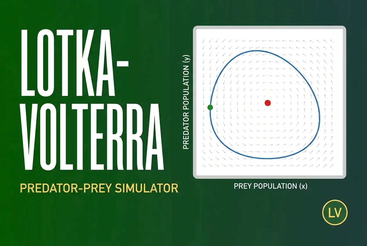
The phase plane plot shows prey on the horizontal axis and predator on the vertical axis. The closed orbit appears as a loop around the coexistence equilibrium (red dot). The initial condition is a green dot. The direction field arrows show the local flow direction.

The time series plot shows both populations on the same axes against time, with prey in blue and predator in red. In the small-amplitude limit, the two curves are out of phase by approximately a quarter of a period; for larger finite-amplitude orbits, the lag deviates from the quarter-period estimate.

Worked examples

Example 1: Classical textbook (alpha=beta=delta=gamma=1)

Setup: Click the Classical textbook preset. The coexistence equilibrium is at x* = 1, y* = 1. The closed orbit passes through x₀ = y₀ = 1.5 (50 percent above the equilibrium) and has a period of approximately 6.48 time units. The simulator reports a maximum conservation error below 1e-4 (well within the green threshold) for the default step size dt = 0.01.

Results: The phase plane shows a closed orbit symmetric in x and y. The time series shows predator peaks following prey peaks. At this finite oscillation amplitude, the lag is not exactly one quarter of a period.

Example 2: Lynx and snowshoe hare (illustrative)

Setup: Click the Lynx and snowshoe hare preset. The coexistence equilibrium is at x* approximately 16.7, y* approximately 22.2. The orbit extends from approximately x = 10.2 to x = 25.4.

This illustrative parameter set produces a period of about 16 time units, longer than the roughly 10-year snowshoe-hare cycle. Because the parameters were not fitted to the observed data, this comparison should not be interpreted as a model-prediction error. The basic model also omits carrying capacity and other important ecological drivers (Krebs, Boonstra, and Boutin 2018).

Results: The orbit has a larger amplitude than the classical case. The detected period of about 16 time units is longer than the observed 10-year snowshoe-hare cycle, but the parameters are illustrative and not fitted to data, so this is not a model-prediction error. The standard Lotka-Volterra model also omits carrying capacity and other important ecological drivers (Krebs, Boonstra, and Boutin 2018).

Example 3: Vertical orbit (low prey growth)

Setup: Click the Vertical orbit preset. The prey growth rate alpha is 0.2, and the predator mortality rate gamma is 0.5. The orbit is taller than it is wide, with the predator variance larger than the prey variance. The coexistence equilibrium is at x* = 5, y* = 2.

Results: The closed orbit has a tall, narrow shape, with predator oscillation amplitude larger than prey amplitude.

Example 4: Horizontal orbit (low predator efficiency)

Setup: Click the Horizontal orbit preset. The predator efficiency delta is 0.05, which is much lower than the default. The orbit is wider than it is tall, with prey variance larger than predator variance. The coexistence equilibrium is at x* = 10, y* = 2.

Results: The closed orbit has a wide, short shape, with prey oscillation amplitude larger than predator amplitude. The predators fluctuate less because the low efficiency means they take longer to convert prey into offspring.

Example 5: Conservation demonstration (small amplitude)

Setup: Click the Conservation demonstration preset. The initial conditions are 5 percent above the coexistence equilibrium (x₀ = y₀ = 1.05). The orbit is small and nearly elliptical, and the period is within 1 percent of the small-amplitude formula 2 times pi divided by sqrt(alpha times gamma).

Results: The conservation error is much smaller than for the larger-amplitude presets. The orbit is small and numerically less demanding, so the absolute conservation error stays well below 1e-13. The detected period is very close to the small-amplitude estimate.

Limits and caveats

• The standard Lotka-Volterra equations do not include a carrying capacity for prey. The lynx-hare preset is illustrative, not a fit to data. A logistic prey term is a candidate v2 feature.
• The simulator enforces the strict positivity of all four rate parameters and the initial conditions. The UI minimum is 0.01 for each value. Inputs at zero or negative are rejected.
• The conservation invariant check measures the absolute error of the first integral C. Values below 1e-4 indicate a well-resolved trajectory and are color-coded green. Values above 1e-2 indicate a need for a smaller step size and are color-coded red.
• The closed-orbit property is exact for the continuous system but approximate for the discrete integrator. The integration error scales as the fourth power of the step size at fixed final time.

Lotka-Volterra simulator vs related ecology tools

The Lotka-Volterra simulator focuses on the simplest two-species predator-prey model.

• Tools for more complex population dynamics (logistic prey growth, Holling Type II functional response, three-species food chains) are future v2 features.
• For Hardy-Weinberg population genetics, see the dedicated Hardy-Weinberg calculator on the biology tools directory.
• For other biology calculators covering cell culture, dose-response curves, and inheritance, see the biology tools page.

Related Resources

References

• Volterra, V. (1926). Fluctuations in the Abundance of a Species considered Mathematically. Nature, 118, 558-560. The original derivation of the predator-prey equations used in this calculator.
• Lotka, A. J. (1925). Elements of Physical Biology. Williams and Wilkins. The independent derivation of the same equations, one year before Volterra.
• National Institute of Standards and Technology. OOMMF Evolvers (Oxs_RungeKuttaEvolve) user guide, RK4 method with 1/15 step-doubling estimator. Reference for the standard 1/15 step-doubling error estimator used in this calculator.
• Krebs, C. J., Boonstra, R., and Boutin, S. (2018). Using experimentation to understand the 10-year snowshoe hare cycle in the boreal forest of North America. Journal of Animal Ecology, 87(1), 87-100. The snowshoe-hare cycle has multiple ecological drivers beyond predator-prey interactions.
• May, R. M. (1972). Will a Large Complex System be Stable? Nature, 238, 413-414. The foundational analysis of the relationship between complexity and stability in model ecosystems, including predator-prey systems.

Frequently Asked Questions