
Cell Viability Dose-Response Calculator
A cell viability dose-response calculator fits a 4-parameter logistic (4PL) curve to (concentration, viability) data using Levenberg-Marquardt nonlinear least squares. The same tool returns the IC50 (or EC50 for activation), Hill slope, top and bottom plateaus, R2, parameter standard errors, a 95% confidence interval on the IC50, an interactive dose-response curve plot, and a pIC50 or pEC50 value.
The math follows the standard pharmacology 4PL model (Prinz 2010; Lyles et al. 2008), with IC50 confidence intervals computed on the log10 concentration scale and then back-transformed.
Cell Viability Dose-Response Calculator
Fit a 4-parameter logistic (4PL) curve to your dose-response data using Levenberg-Marquardt nonlinear least squares. Returns the IC50 (or EC50) with 95% confidence interval, Hill slope, plateaus, R2, and a fitted dose-response curve plot. Includes 6 synthetic worked examples based on published assay contexts.
Input data
Enter your (concentration, viability) pairs. The vehicle control (x = 0) is shown for reference but is not used in the 4PL fit.
Inhibition: viability decreases with dose (standard cytotoxicity). Activation: viability increases with dose (e.g., growth factors).
| Conc (uM) | Viability (%) |
|---|
Advanced: fixed parameters
Fixed parameters reduce the degrees of freedom for SE/CI computation. SE on a fixed parameter is exactly 0.
Output
Press Fit 4PL curve to compute the IC50, Hill slope, and curve parameters.
Dose-response curve
Observed 4PL fit IC50
Fitted parameters
Worked examples reference
The 6 presets above are synthetic dose-response curves based on published assay contexts and reported potency ranges. The data are generated from the listed 4PL parameters; the published reference is the source for the cell line, drug, assay, and approximate IC50, not for the exact tabulated values.
| Cell line | Drug | Assay | Time | Unit | Model IC50 |
|---|
✔ The 4-parameter logistic is the standard dose-response model for pharmacology, with top, bottom, Hill slope, and IC50 as the four parameters.
✔ This calculator fits a 4PL curve to your (concentration, viability) data using Levenberg-Marquardt nonlinear least squares, and reports the IC50 with a 95% confidence interval on the log scale.
✔ Switch the response direction to fit activation curves and get EC50, EC10, and EC90 instead of the IC variants.
✔ Use the fixed-asymptote option when you have independent confirmation of the top or bottom value, for example from control wells.
✔ The 6 worked examples cover common cancer cell line and drug combinations and recover the listed model parameters closely when fit.
What is a cell viability dose-response curve?
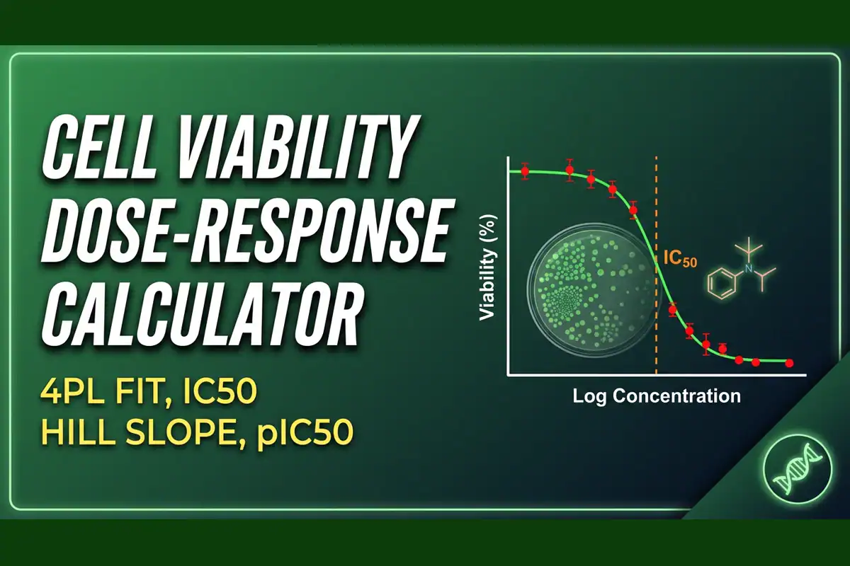
A cell viability dose-response curve plots the percentage of viable cells (y axis) against the logarithm of the drug concentration (x axis), after a fixed exposure time. For a standard cytotoxicity assay, the curve has a sigmoidal shape: viability is high at low doses (the vehicle control, where no drug is present) and drops to a low plateau at high doses (where the drug has killed most cells).
The dose at which viability is exactly 50% of the way between the top and bottom plateaus is called the IC50 (inhibitory concentration 50). For activation assays, where the treatment increases viability, the equivalent value is the EC50 (effective concentration 50).
The standard mathematical model for this curve is the 4-parameter logistic (4PL), also called the Hill-Langmuir equation or simply the Hill equation. The 4PL captures the four features that any sigmoidal dose-response curve has: the top asymptote, the bottom asymptote, the steepness of the transition, and the position of the inflection point.
This calculator fits the 4PL to a single dataset of (concentration, viability) pairs and reports the four parameters along with derived quantities like R2, the 95% confidence interval on the IC50, and the working range (IC10 and IC90).
The 4PL is a common workhorse model in pharmacology and is supported by tools such as GraphPad Prism and the R drc package. It is often a reasonable choice for receptor binding, cell viability, enzyme inhibition, calcium flux, and other pharmacology assays where the response is monotonic in dose.
For non-monotonic data, such as hormesis or biphasic responses, you need a different model, and this calculator may give a poor fit and warn you with a low R2.
How to use the calculator
- Pick a worked example (optional). Six presets are available covering common cancer cell line + drug combinations: HeLa + Doxorubicin, HEK293 + Staurosporine, MCF-7 + Paclitaxel, A549 + Cisplatin, HCT116 + 5-Fluorouracil, and HepG2 + Sorafenib. Each loads synthetic dose-response data generated from the listed 4PL parameters.
- Choose the response direction. Inhibition mode is the default for cytotoxicity assays, where viability decreases with dose. Activation mode is for growth factors and similar assays where viability increases with dose. The labels switch from IC50 / IC10 / IC90 to EC50 / EC10 / EC90 automatically.
- Pick the concentration unit. The presets use the unit reported in the source publication, typically nM for kinase inhibitors and uM for chemotherapeutics. The unit applies to both the table data and the IC50 output. Changing the unit rescales the table values; the fitted IC50 rescales too.
- Edit the data table. Each row is a (concentration, viability) pair. The first row is the vehicle control (x = 0); the next 7 are positive doses. Blank concentration or viability fields are rejected with a clear error message.
- Optionally fix the top or bottom asymptote. Open the Advanced section and enter a value for A or D if you have independent confirmation. The degrees of freedom for SE and CI computation drop accordingly.
- Press Fit 4PL curve. The calculator runs Levenberg-Marquardt, reports the IC50 with 95% CI, the Hill slope, the plateaus, R2, pIC50, and draws the fitted curve.
The 4-parameter logistic equation
The 4PL model used in this calculator is:
Where x is the drug concentration (positive, in the unit you selected), y is the response (viability %), and the four parameters are:
- A (top asymptote) is the response as x approaches 0, expected to equal the vehicle control value (typically 100% for normalized data).
- D (bottom asymptote) is the response as x approaches infinity, expected to equal the maximum-effect value (typically 0% for full inhibition).
- B (Hill slope) is the steepness of the curve at the inflection point. B is positive for inhibition and negative for activation in this linear-concentration form. Typical values for cytotoxicity assays are 1 to 3.
- C (IC50 or EC50) is the inflection point, the dose at which y = (A + D) / 2. For a normalized curve with A = 100 and D = 0, this is the dose at 50% viability.
The sign of B deserves a special note because it is a frequent source of confusion. The slope at the inflection point is (A minus D) times B divided by 4C. For an inhibitory curve (response decreases with dose), the slope is negative. Since (A minus D) is positive and C is positive, this requires B to be positive.
If you have seen dose-response fits where the Hill slope is reported as a negative number, the calculation used a different equation form, typically the GraphPad log-concentration form: 10 to the ((x minus LogIC50) times HillSlope), where HillSlope is positive in the log form.
Both conventions are valid; this calculator uses the linear-concentration form because it keeps all four parameters in a single consistent sign.
IC50 versus EC50 and the relative-versus-absolute distinction
The reported value C from a 4PL fit is the dose at response equal to (A + D) / 2, which is called the relative IC50. For normalized data with A = 100 and D = 0, the relative IC50 is also the dose at 50% viability, which is what most pharmacology papers mean when they write “IC50“. This is the value the calculator reports.
The absolute IC50, sometimes called the “true IC50“, is the dose at 50% of the zero-dose response, regardless of the asymptotes. It only equals the relative IC50 if D = 0 (full inhibition).
For curves where D is not 0, for example when a small fraction of cells survives at saturating drug, the absolute IC50 and the relative IC50 differ. The difference is usually small but matters for publication.
The calculator reports the relative IC50 with a footnote noting the convention; if you need the absolute IC50, compute it from the reported A, D, and C by solving y = 0.5 A for x:
For the common case of A = 100 and D = 0, this reduces to C (the relative IC50 equals the absolute IC50). For D nonzero, the absolute IC50 is shifted away from C.
Confidence interval on the IC50
The 95% confidence interval on the IC50 is computed on the log scale using the delta method, then back-transformed. This approach gives an asymmetric interval on the linear scale that is closer to the true sampling distribution of an IC50 than a symmetric interval on the linear scale. The formula is:
Where t(0.975, n minus p) is the 97.5th percentile of Student’s t distribution with n minus p degrees of freedom (n is the number of data points, p is the number of free parameters), and SE(log10 C) is the standard error of log10 C from the LM covariance matrix. The interval is back-transformed to the linear scale with 10 to the x, giving lower and upper IC50 bounds.
For a typical 7-point dose-response curve with 4 free parameters, n minus p = 3 and t(0.975, 3) is approximately 3.18, much wider than the normal-approximation 1.96. This is intentional: with only 3 residual degrees of freedom, the sample variance is poorly estimated, and a wider CI is more honest. As n increases, t approaches 1.96, but you should still use the t critical value for the typical small dose-response dataset.
If n minus p is less than 2 (n less than 6 for a free 4PL fit), the calculator suppresses the SE and CI rather than report a wildly inflated value, and emits a yellow warning that the dataset is too small for reliable inference. This is a common situation in pilot screens, and the workaround is either to add more points, fix one or more parameters, or pool the standard deviation across biological replicates.
Working range: IC10 and IC90
The IC10 and IC90 (or EC10 and EC90) give the dose range over which the drug is doing something useful: above IC10, the drug is starting to show measurable effect; below IC90, the drug is not yet at saturating effect.
The two values are useful for planning follow-up experiments, for example choosing a sub-cytotoxic dose for a synergy screen or a saturating dose for a positive control. From the 4PL fit:
IC90 = C × 91 / B
For B = 1, IC10 and IC90 are one decade below and above C, the familiar log-symmetric spread. For B = 2, the spread is half a decade on each side, a steeper curve. For shallow B (less than 0.5), the spread is more than two decades, and the curve looks more like a smooth ramp than a sharp threshold.
The Hill slope is therefore a measure of cooperativity: high B means the drug response switches on sharply over a narrow dose range, low B means a gradual response.
What is pIC50?
The pIC50 is the negative base-10 logarithm of the IC50 expressed in molar:
For an IC50 of 5 micromolar (5e-6 M), pIC50 = -log10(5e-6) = 5.30. pIC50 is widely used in pharmacology because it compresses the wide concentration range (pM to mM) into a single number that is closer to normally distributed, which makes it easier to compare compounds statistically. A higher pIC50 means a more potent compound (lower IC50). For activation curves, the same definition gives pEC50.
Fixed asymptotes: when and how
The Advanced section lets you fix the top asymptote A or the bottom asymptote D to a known value. Fix A when you have independent confirmation of the vehicle control, for example from a separate cell-count or an orthogonal assay. Fix D when you know the maximum effect of the drug, for example from a saturating-dose positive control.
Fixed parameters are handled by a reduced-parameter Levenberg-Marquardt: the fixed parameter is removed from the iteration vector entirely, the free parameters are fit, and the standard error on the fixed parameter is exactly 0. The degrees of freedom for SE and CI computation drop accordingly: a fixed A means nFree = 3; fixed A and D means nFree = 2.
Use fixed asymptotes with care. Over-constraining the fit (for example, fixing A = 100 when the actual top is 95 due to assay background) biases the other parameters and inflates the residual variance.
The calculator suppresses the bound warnings for fixed parameters (since they are at their user-specified value, not at a fitted bound) and emits neutral notes of the form “top-fixed = 100” or “bottom-fixed = 0”. If you see a poor R2 after fixing a parameter, the constraint is likely too tight.
The 6 worked examples
The 6 presets cover common cancer cell line and drug combinations, drawn from published pharmacology papers and large kinome scan databases. Each preset is a synthetic dose-response curve generated from the listed 4PL parameters.
The published reference is the source for the cell line, drug, assay, time, and approximate IC50, not for the exact tabulated values. The fit should recover the model parameters to within about 1 to 2% on each preset.
| Cell line | Drug | Assay | Time | Unit | Model IC50 | Reference |
|---|---|---|---|---|---|---|
| HeLa | Doxorubicin | MTT | 24 h | μM | 0.5 | Kalyanaraman 2002 |
| HEK293 | Staurosporine | CellTiter-Glo | 24 h | nM | 50 | Karaman 2008 kinome scan |
| MCF-7 | Paclitaxel | MTT | 72 h | nM | 5 | Liebmann 1993 |
| A549 | Cisplatin | MTT | 48 h | μM | 5 | Fennell 2016 NSCLC panel |
| HCT116 | 5-Fluorouracil | MTT | 72 h | μM | 5 | Tie 2018 colorectal panel |
| HepG2 | Sorafenib | MTS | 48 h | μM | 5 | Wilhelm 2004 |
Try fitting each preset and comparing the recovered IC50 to the model IC50 in the table. The fit should agree to 3 significant figures (R2 = 1.0000) because the data are exact 4PL outputs from the listed parameters.
In real data, the agreement depends on the noise level: typical MTT or CellTiter-Glo data with biological triplicates give R2 of 0.98 to 0.99 and IC50 within 10 to 20% of the truth.
When to use this calculator
Five common use cases are below. The calculator is for a single (concentration, viability) dataset at a time. Multi-curve comparison and combination-index analysis are out of scope.
- Pharmacology coursework. When you run a dose-response lab (MTT, CellTiter-Glo, alamarBlue) and need to report the IC50 with a 95% confidence interval in a lab report or thesis figure.
- Cancer drug screening pre-analysis. When you have a 96-well plate of dose-response data and need a quick IC50 readout before submitting the raw data to GraphPad Prism, R, or the
drcpackage for the final analysis. - Single-experiment quick fit. When a collaborator asks for the IC50 from one experiment and you want a defensible number (with CI) in 30 seconds rather than spinning up a full R session.
- Assay comparison. When you ran the same drug on the same cell line in two assays (MTT vs CellTiter-Glo) and want to compare the recovered IC50 and Hill slope to flag assay-specific artifacts.
- Working-range planning. When you need the IC10 and IC90 to choose doses for a downstream experiment, for example a synergy screen or a time-course study.
How this fits with the other cell biology calculators
The Cell Viability Dose-Response Calculator sits alongside the other cell biology tools.
- For a single cytotoxicity readout at one dose, the Annexin V/PI Apoptosis Calculator covers the early/late apoptosis and necrosis breakdown from a flow cytometry experiment.
- For population growth curves, the Cell Doubling Time and PDL Calculator handles the time-course side.
All three tools share the same pedagogical math + interactive UI design. The full set lives at the cell biology calculators hub.
Sources and further reading
The 4PL model, the Levenberg-Marquardt algorithm, the delta-method confidence interval on the log scale, and the dose-response assay conventions used in this calculator are drawn from the following peer-reviewed sources.
- Prinz H (2010). Hill coefficients, dose-response curves and allosteric mechanisms. Journal of Chemical Biology 3: 37 to 44. doi:10.1007/s12154-009-0029-3
- Lyles RH, Poindexter C, Evans A, Brown M, Cooper CR (2008). Nonlinear model-based estimates of IC50 for studies involving continuous therapeutic dose-response data. Contemporary Clinical Trials 29: 878 to 886. doi:10.1016/j.cct.2008.05.009
- Giraldo J, Vivas NM, Vila E, Badia A (2002). Assessing the (a)symmetry of concentration-effect curves. Pharmacology & Therapeutics 95: 21 to 45. doi:10.1016/S0163-7258(02)00223-1
- Ritz C, Baty F, Streibig JC, Gerhard D (2015). Dose-Response Analysis Using R. PLOS ONE 10(12): e0146021. doi:10.1371/journal.pone.0146021
- Mosmann T (1983). Rapid colorimetric assay for cellular growth and survival: Application to proliferation and cytotoxicity assays. Journal of Immunological Methods 65: 55 to 63. doi:10.1016/0022-1759(83)90303-4
- Riss TL, Moravec RA, Niles AL, Duellman S, Benink HA, Worzella TJ, et al. (2013). Cell viability assays. NCBI Bookshelf NBK144065. NBK144065
Frequently asked questions
The IC50 is the drug concentration that reduces cell viability to 50 percent of the vehicle control. In a 4-parameter logistic (4PL) fit, the IC50 is the inflection point of the fitted curve, where the response equals (A + D) / 2. For a normalized curve with A=100 percent and D=0 percent, the IC50 is the concentration at 50 percent viability. For activation curves, the equivalent value is the EC50.
IC50 (inhibitory concentration 50) refers to the dose at 50 percent inhibition, where the response decreases with dose. EC50 (effective concentration 50) is the dose at 50 percent of the maximum effect in either direction, and is used for activation curves where the response increases with dose. The math is the same; only the sign of the Hill slope and the labelling differ.
The Hill slope (B) is the steepness of the dose-response curve at the inflection point. A Hill slope of 1 gives a symmetric curve on a log-concentration axis; values greater than 1 give a steeper curve; values less than 1 give a shallower curve. In this calculator, the sign of B is positive for inhibition and negative for activation, following the linear-concentration form of the 4PL equation.
The 95 percent CI on IC50 is computed by delta method on the log10 scale, using the t critical value for the residual degrees of freedom (n minus p, where p is the number of free parameters). The formula is log10(IC50) plus or minus t(0.975, df) times SE(log10 IC50), then back-transformed with 10 to the x. This approach gives asymmetric CIs on the linear scale that are closer to the true log-normal sampling distribution of IC50.
Fix the top asymptote A when you have independent confirmation that the vehicle control produces 100 percent viability, for example from a separate control well count. Fix the bottom asymptote D when you know the maximum effect, for example from a positive-control cytotoxic at saturating dose. Fixed parameters reduce the degrees of freedom for SE and CI computation. The standard error on a fixed parameter is exactly 0.
4PL has four parameters: top, bottom, Hill slope, and IC50. 5PL adds a fifth parameter, asymmetry, that allows the curve to have different slopes on either side of the inflection. 4PL is the standard for pharmacology dose-response; 5PL is used when the curve is clearly asymmetric, which is rare for simple receptor binding or viability assays. This calculator uses 4PL because it covers many routine monotonic pharmacology datasets with fewer degrees of freedom.
pIC50 is the negative base-10 logarithm of the IC50 in molar. For example, an IC50 of 5 micromolar (5e-6 M) gives pIC50 = -log10(5e-6) = 5.30. pIC50 is used in pharmacology because it transforms a wide concentration range into a compact logarithmic scale, which often makes compound potency values easier to compare statistically.
Several common causes: (1) the data are not actually 4PL-shaped, e.g., biphasic response, hormesis, or non-monotonic dose-response. (2) too few points at the upper or lower plateau, so the asymptote estimates are pulled by outlier data. (3) a single outlier that pulls the fit; consider removing it or running with a robust fitter. (4) the dose spacing does not cover enough log-range around the IC50. The calculator reports a residual standard error and R-squared; if R-squared is below 0.95, the 4PL may not be the right model.
This educational tool was developed by BioExplorer for pharmacology coursework, cancer drug screening pre-analysis, and single-experiment quick IC50 readout. It uses a deterministic 4-parameter logistic (4PL) regression via Levenberg-Marquardt nonlinear least squares, with the 95% confidence interval on IC50 computed by delta method on the log scale.
The calculator is open and free to use. Source code and test suite are available in the published package. If you need a more flexible or research-grade dose-response tool, consider the R package drc (Ritz et al. 2015) or GraphPad Prism, which support 5PL, Gompertz, and other model forms plus multi-curve comparison.
Cite this page
BioExplorer. (2026, September 30). Cell Viability Dose-Response Calculator. https://www.bioexplorer.net/cell-viability-dose-response-calculator/